Week 7 - Proportional Symbol Maps

The displayed map was created as part of the University of West Florida Online GIS Certification program class, Cartographic Skills, (GIS 3015/L) for the Week 7 lab exercise: Proportional Symbol Maps. The map was generated using GIS ArcMap software and then exported to Adobe Illustrator for finishing and adding the proportional circles.



I decided to try something different this time by making the mapped area white and the background gray in hopes that it would add figure-ground appeal. I didn't like how the map first looked with black borders so the border was lightened several shades. When I started adding my proportional circles, I intended to use opaque black circles thinking they'd stand out really well. However, using opaque circles presented a problem in that a lot of the countries were very small and also I felt it was important to try to preserve the country labels since that information would be useful to a map reader. Placing some of the larger circles, such as for Italy and France, sealed the deal because so much of the border was wiped out by the symbol and I did not like the way it looked. So I changed the symbol to dark gray and then set a transparency so borders and labels could be seen. In the end I chose a transparency level of 90% opaqueness which is almost full opaqueness but seems to retain the ability to see the necessary information. I also moved a lot of the country labels to places where they could more easily be read adding leader lines as needed. I did add the amount for Germany to my map although I'm not sure we were supposed to. For the one country that I found that was not a wine producing country I shaded the entire country with a 50% white to black gradient which allows it to stand out but not overwhelm the other parts of the map.

For the legend I chose to create a set of six symbols based on applying something close to the optimal method for choosing the first 5 symbols and then adding a sith in the large gap between two symbols.

Creating the circles and getting them into position and working them in with the labels was time consuming and painstaking as was creating the legend.

Module 6 - Choropleth Mapping

The posted maps were completed as part of the Week 6 lab for the University of West Florida Online GIS Certification program class, Cartographic Skills (GIS 3015/L), and demonstrate techniques in choropleth mapping.

Color Choropleth Map
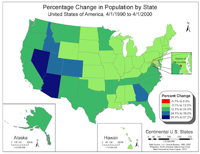
The first map is a color choropleth showing the population change by state for the United States from April 1, 1990 to April 1, 2000. The map was generated using ArcMAP and exported for finishing in Abobe Illustrator (CS4).


Generating the map in ArcMap was fairly straightforward process. I actually created 4 data frames to get the Alaska, Hawaii and DC insets. I used a contrasting red for the negative population growth, not realizing only DC was going to show that number. Probably could have avoided doing so, but I thought that was an interesting thing to highlight. I tried to use the Color Brewer web site but found the light color not to my liking for the map because too many border states were light and seemed to fade into the background.

Black and White Choropleth
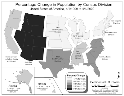
The next map is another choropleth showing population change, however this time by U.S. Census Divisions. The idea was to take the first choropleth map and alter it in Adobe Illustrator to create a new map with new information, divisions and such.

Creating the map was actually pretty fun though somewhat painstaking. The project first required running calculations from the state population data to obtain division data. I used Excel for the task printing out my work and it helped me organize the ideas for how I would display the map and make sure I selected the correct states for each division.

Knowing that the map would be gray-scale, I wanted to try to create a visual separation on the divisions and decided to "float" them away from each other. Since this is a thematic map, I feel that doing so is acceptable because of the visual effect it adds to the thematic goal of the map. However, in order to be able to move a division, I had to group all the states in the division into one group layer to make it easier to select a division, adjust it's position then select another division. Grouping also made coloring the states a snap as I could just select the group and hit the swatch color for that class which I set up beforehand. Trisha, thanks for reminding us to re-watch that Abode tutorial on Layers and Groups it helped immensely.

Al in all I'm pretty happy with both maps.

Module 5 - Map Composition

The following map was created for the Map Composition module of the University of West Florida Online GIS certification course, Cartographic Skills (GIS 3015L). The map was created using Adobe Illustrator (CS4).




The goal of the assignment was to take various components of a typical thematic map and organize them in a cohesive and aesthetically effective manner to convey the map's information. The layout presented above accomplishes the goal by focusing on the thematic map which had to be enlarged to scale and then balanced to the other elements (insets, legend, scale bar, north arrow). It was quite a challenge to get the elements arranged correctly and I was only pleased with the composition after re-positioning the Florida inset in the bottom corner with the US map above it creating a "stacked building" effect on the left side that settles the viewers gravitational unease. Originally, the legend had a border as well, but I realized it really did not need it because it was in-kind part of the main map at that point. The insets were given a color fill to create contrast to the main map, as well as to each other to seal the deal. At that point, a defined diagonal framing of the main map was created that balanced the diagonal shape of the part of Florida being highlighted. I considered changing color schemes for the thematic map, but the compositional elements made it unnecessary. However, pretty much every element in the map was re-sized in some format (i.e. the scale was halved in thickness and a segment removed to shorten it to scale) and all the type was changed to Ariel and re-sized to various point sizes.

My best friends in Illustrator were the Layers frame which I used religiously to lock and hide objects and layers and the Direct Selection tool which made selecting the maps as one piece very easy. I had problems using the Scale tool until I realized it was easier to use when the image was enlarged.

Module 4: Typography

The map shown below of the middle section of the Florida Keys was created for the Typography lab for the University of West Florida on-line GIS certification program class, Cartographic Skills (GIS 3015/L).

The map was not created using ArcGIS but rather was created in Adobe Illustrator. Students were given the map outline and had to use their understanding of typography rules for map-makers to locate and label various features in this area of the keys. I can honestly say that doing so proved tremendously frustrating as there was a lot about the Adobe program that was very foreign to me and not easily understood. For example, I wanted to color in the state park and country club land areas in green, but was at a loss how to easily fill an area. The closest I came was using a paint-like feature which took forever, created multiple objects, and had zero precision. I'm sure there's a better way to do it, but the Adobe help to say the least is least helpful. I now strongly regret not downloading a trial of this version before starting the course.

I do feel like I learned quite a bit about using the program. The zoom feature was very useful in placing labels and I did arch a few of them to get them to fit in to tight places. I only used two types for the elements, one serifed and one sans serif. There were elements and rules followed for this map that I did not pay attention to previously and hope to keep in mind for the next labs.

Module 3 - Data Classification Lab (Escambia County, FL)

The following maps were created for the University of West Florida 2010 GIS Certification program course, Cartographic Skills (GIS 3015/L) using ArcGIS. The maps depict the African population percentage of Escambia, FL based on year 2000 census data.



The first map shows four chloropleth maps of Escambia county using different data classification methods: Equal Intervals, Quantile, Standard Deviation and Natural Breaks.

Which Classification best represents the data and why?

To answer the question I looked at the way the data was spread using the Classify button under the Symbology tab and noted the leftward skew of the data indicating that the majority of census tracks in Escambia county have low population percentages of Africans (36 of 58 are roughly 25% or less) while three have very high percentages (86%, 88.1%, 95.6%). As such, the best map of the data should highlight these two extremes, especially the high percentage tracks.

Examining the distributions created by each of the four Data Classification methods helped to identify which classification best displayed those aspects. The Quantile method was rejected because it spanned too great a range of values, 44.6 – 95.6 (over 50% of the total range), into one Class break. The Standard Deviation method was rejected because the distribution of the data was not normally distributed. The Natural Break method was rejected because it did not isolate the high percentage values, even after adding up to 13 breaks.



The Equal Interval classification seemed the best fit because its legend isolated most of the tracks under 25% into one interval and had a higher starting percentage for the upper range, much closer in value to the high percentage tracks, making them easily identified on the map and providing a better indicator of their outlying nature.